My Work #1: Momentum-space lattices
- Atom-optics simulator of lattice transport phenomena
- Eric Meier, ME, and Bryce Gadway
- Phys. Rev. A 93 (2016)
- arXiv:1601.05785
In the spirit of trying to explain complicated physics nonsense (the point of this site), I’ll start with my own work in the Gadway lab. In this series of posts, I will explain each of my studies at a more easily digestible level, giving a short 1-2 paragraph summary and filling in the minimum background necessary. However, this first post might need a bit more background…
I’ve tried to write this at the level of a physics undergraduate. Jargon is italicized.
Summary
Eminent scholars Alex, Eric, and Bryce make lattices in momentum space for cold atoms, instead of the usual real-space optical lattice setup. This technique gives individual control over each tunneling amplitude, tunneling phase, and site energy of the lattice. They create a few simple lattice systems to demonstrate their control over their lattice: a 1D lattice, a 1D lattice with a tilt, and a 1D lattice with a tunneling “echo”: suddenly switching all the tunnelings to be negative halfway through.
To be honest, momentum-space lattices fill a small niche in the field of cold atoms in optical lattices. While we do have very precise control over our lattice parameters compared to real-space lattices, we are usually forced to start our experiments with all of the atoms in just one lattice site: atoms are initially at rest, so they are all in the zero momentum “lattice site.” This is normally not close to the ground state (or any eigenstate) of the lattice system, so our experiments could be considered really out-of-equilibrium. This sort of measurement has limited utility: for example, probing eigenstates is… hard.
Detail on momentum-space lattices
At its core, my work so far has been exploring what we could do with atoms in a momentum-space lattice setup (Bryce’s brainchild, proposed in a previous work, arXiv:1601.05818). In a traditional “real-space” optical lattice setup, a standing wave of light (laser hitting a mirror) creates a periodic lattice potential for atoms that looks like a bunch of potential wells separated in space. (The light gives an intensity-dependent shift to the atoms’ energy levels - AC Stark effect - trapping the atoms at the peaks of the standing wave.) Atoms can then tunnel through the barriers between wells, and you can do things to the lattice like apply a tilt, shake it, or make the wells really deep to restrict tunneling. The point of this whole thing is quantum simulation: atoms in this optical lattice behave like any quantum particles in a lattice, so you can use this system to study, for example, electrons in a crystal.
Our approach is to make a similar periodic structure, but instead of potential wells separated in position, ours are separated in momentum. To create these momentum states, we shine on our atoms a laser with wavelength $\lambda=1064~$nm and wavenumber $k=2\pi/\lambda$. Because an atom can only absorb one photon and then emit one photon at a time, the atoms can only get a momentum kick of two times the photon momentum: $\pm 2 \hbar k$. So, the atoms’ momentum is restricted to discrete momentum states $p_n = 2 n \hbar k$ for integer $n$. The atoms are just free particles, so the energy of these states is just the kinetic energy $E_n = \dfrac{p_n^2}{2m}$ (where $m$ is the mass of the atom).
To make a lattice out of these states, we need to couple them. To couple two states $n$ and $n+1$, we do what any atomic physicist would do and apply a laser field at the exact energy difference between the states ($E_{n+1}-E_n$)… or we would if the energy difference weren’t so small (corresponding to frequencies on the kHz scale). Instead, we use two lasers with a frequency difference that matches the energy difference between the states (this two-laser method is called a Raman transition). Atoms in state $n$ are then connected to state $n+1$ and population oscillates between the two states (Rabi oscillations). This is a two-site lattice, and we can easily couple more states by putting more pairs of lasers with different frequencies onto the atoms.
The physical implementation is very simple: a pair of acousto-optic modulators (AOMs). These devices are small crystals that can take in some radio frequency (around 80 MHz) and put that frequency onto a laser passing through. So, we just hook this to an arbitrary waveform generator which can output a bunch of different frequencies. The workflow is thus: we generate the actual waveform in Mathematica by adding up our desired frequencies, sampling that discretely, and outputting it to a text file. Then we pass that to the arbitrary waveform generator, which generates an oscillating voltage signal that then goes through some amplifiers into our AOM, which writes the frequencies onto the laser. The laser then hits the atoms and addresses the transitions between momentum states, creating the MOMENTUM-SPACE LATTICE. (There’s a small caveat here: because the transition frequencies between momentum states are on the kHz scale, we need to use two AOMs: one to add 80 MHz and the transition frequencies, and another to take away the 80 MHz.)
To control lattice parameters, we just change the different parameters of the lasers. To control the “tunneling amplitude” or how fast the atoms oscillate between states, we just change the power in the lasers. To add a “tunneling phase” or a phase onto the atoms’ wavefunction as they tunnel, we just put a phase onto the laser. Finally, we can control the “site energy” by detuning the laser frequency. A feature of our system is the possibility to just cut off the lattice abruptly, making “hard wall” boundaries. This is in contrast to real-space lattices, where the lattice just keeps going on and on.
For measurement, we do the most basic cold atom technique: drop the atoms, or time-of-flight. By releasing any trapping lasers, the atoms fall due to gravity. Because we do the momentum stuff perpendicular to gravity, atoms in different momentum states start flying apart, and we can take a picture when they’re fully separated to read out how much population is in each state.
The actual “picture taking” method we use is absorption imaging, which means we send in a weak laser beam which is resonant with some transition of the atoms. The atoms absorb photons, get excited to some higher state, and get blasted away in the process. The laser then goes onto a CCD camera, and we take a picture showing the shadows of the atoms, from which we can back out how many atoms were in each location.
Three quick experiments
The three lattices we made in this paper were:
- Flat lattices with 21 sites (states $n=-10$ to $10$) and 5 sites ($n=-2$ to $2$)
- 21 site lattice with a tilt to the site energies.
- 21 site lattice with all tunnelings flipping sign after some time (adding a tunneling phase of $\pi$)
I just realized, over 3 years later, that these three experiments all show very similar results: population traveling from the initial site ($n=0$) and coming back. The physics behind the three are completely different, though.
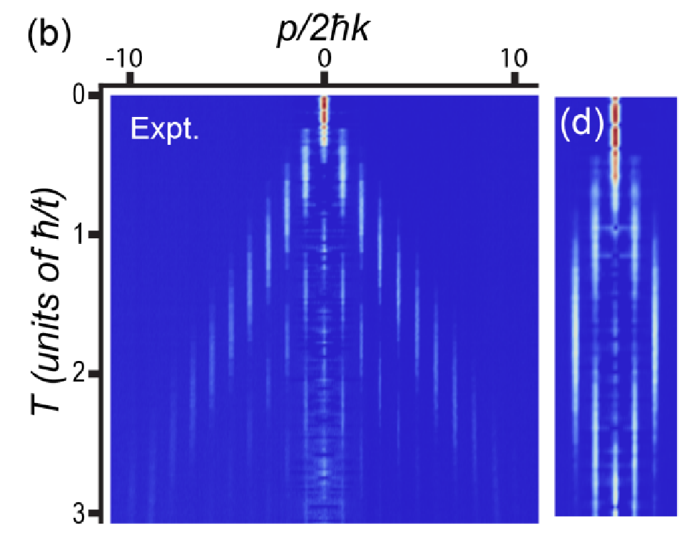
A lattice that is as ordinary as it gets: 21 sites on the left, 5 sites on the right. Atoms begin in the center at $n=0$, and spread out as time progresses (downward vertical axis). In the 5 site case, atoms hit the end of the lattice and come back! This demonstrates our ability to make “hard walls” in the lattice, which has been pretty helpful in some of our studies!
One thing to note is that each horizontal line in this plot is a separate data run (actually an average of several). Our measurement destroys the BEC, so we need to repeat the experiment many times at different times to see the full motion.
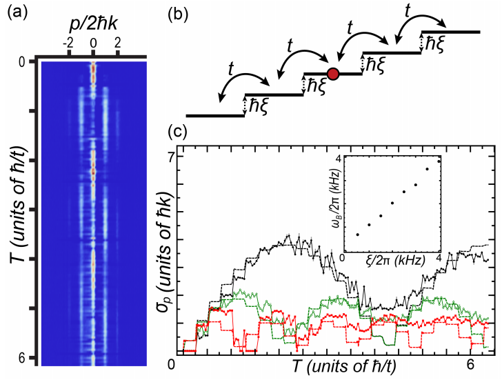
A lattice with a tilt: each site is $\Delta E = \hbar\xi$ (this choice of variable was terrible) away from its neighbors. Classically, this is putting a ball on a slope: it rolls downhill. In the quantum world and in a lattice, atoms don’t just keep moving downhill but instead show oscillations, in a great display of how weird the quantum world can be. These Bloch oscillations are a byproduct of the periodic structure of the lattice, and the oscillation frequency depends directly on the magnitude of the tilt: fig. (c) shows us tilting at three different values.
An aside: Usually for real space lattices people talk about the band structure of the lattice, or how the energy of the lattice states depend on the momentum, $E(k)$. This is periodic like the position, so it results in oscillations. In our confusingly-named momentum-space lattice, we can still think about band structure, but at one extra level of abstraction: because our sites are spaced in momentum, perhaps the band structure should then be the Fourier transform… position? This is generally just too confusing to talk about, so I just say it’s $E(k)$ or $E(q)$ anyway ($q$ is quasimomentum, or momentum in a lattice).
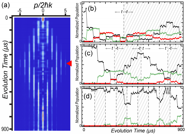
Finally, we switched all the tunneling phases halfway through to show two very nice aspects of our momentum space setup: we can control tunneling phases (important for studying topology, which we later did!), and we can control lattice parameters precisely as a function of time. Figs. b-d show faster tunneling switching, until it’s so fast that atoms don’t have the change to move before they get turned around.
This I think was the birth of me and Eric’s obsession with designing and making figures. Look at that shaded area - simple and elegant!
Conclusion
This post was too long. I wanted to make it detailed, but I made it stupidly long and betrayed my vision of a bare-bones summary of the paper. Hopefully I can refer back to this post for background on momentum-space lattices, though.
P.S.: I’m not entirely sure about the legality/convention that I should use with figures from papers. I think I’ll just go ahead and grab figures and tack on some citations.